Usage

Configuration

All the parameters in the code are specified through a parameter file. An example file can be found in configs/config_example.yaml. All the parameter fields should be self explanatory when familiar with the paper release (TODO: link to arxiv)

 black_hole:
  M: 1e8 # solar masses
  mdot: 0.5 # Eddington units
  spin: 0.0 # spin parameter (-1,1)

radiation:
  relativistic: true 
  f_uv: auto
  f_x: 0.15
  n_r: 1000 # number of bins in the disk
  disk_r_in: 6.0
  z_xray: 0.0
  disk_height: 0.0
  mu_nucleon: 0.61
  mu_electron: 1.17
  xray_opacity: boost 
  tau_uv_calculation: no_tau_uv 
  disk_integral_rtol: 1e-3
  wind_interpolator:
    update_grid_method: "average"
    vacuum_density: 1e2
    nz: 500
    nr: auto 

grid:
  r_min: 6.0
  r_max: 50000.0
  z_min: 0.0
  z_max: 50000.0

initial_conditions:
  mode: CAKIC 
  r_in: 50.0
  r_fi: 1500.0
  n_lines: auto
  log_spaced: true
  z0: 0.0 # Rg
  K: 0.03
  alpha: 0.6
  use_precalculated: true # use cached results

integrator:
  n_iterations: 5
  atol: 1e-8
  rtol: 1e-3
  save_path: "./example"

Running

To run the specified parameter file, we do

using Qwind
model = Model("configs/config_example.yaml")
iterations_dict = Dict()
run!(model, iterations_dict)

The iterations_dict stores information about each iteration of the density grid, so we know how the wind properties and radiation field are changing throughout iterations.

Running in parallel

The code automatically runs with all available cores to Julia. The number of cores that Julia can use can be specified as a launch flag, eg

julia -p 6

will launch Julia with 6 cores. Alternatively, we can make us of the Distributed package,

using Distributed
addprocs(5)

Reading the results

In the example above, the results will be stored in ./tests/results.hdf5. A series of functions are built into QWIND to facilitate reading different data of interest.

Streamlines

streamlines = Streamlines("example/results.hdf5");

We can then easily plot them through

using PyPlot

fig, ax = plt.subplots()
for sl in sls
    ax.plot(sl.r, sl.z, linewidth=1)
end
ax.set_xlim(0,2500)
ax.set_ylim(0,2500)
ax.set_xlabel(L"$R$ [ $R_g$ ]")
ax.set_ylabel(L"$z$ [ $R_g$ ]")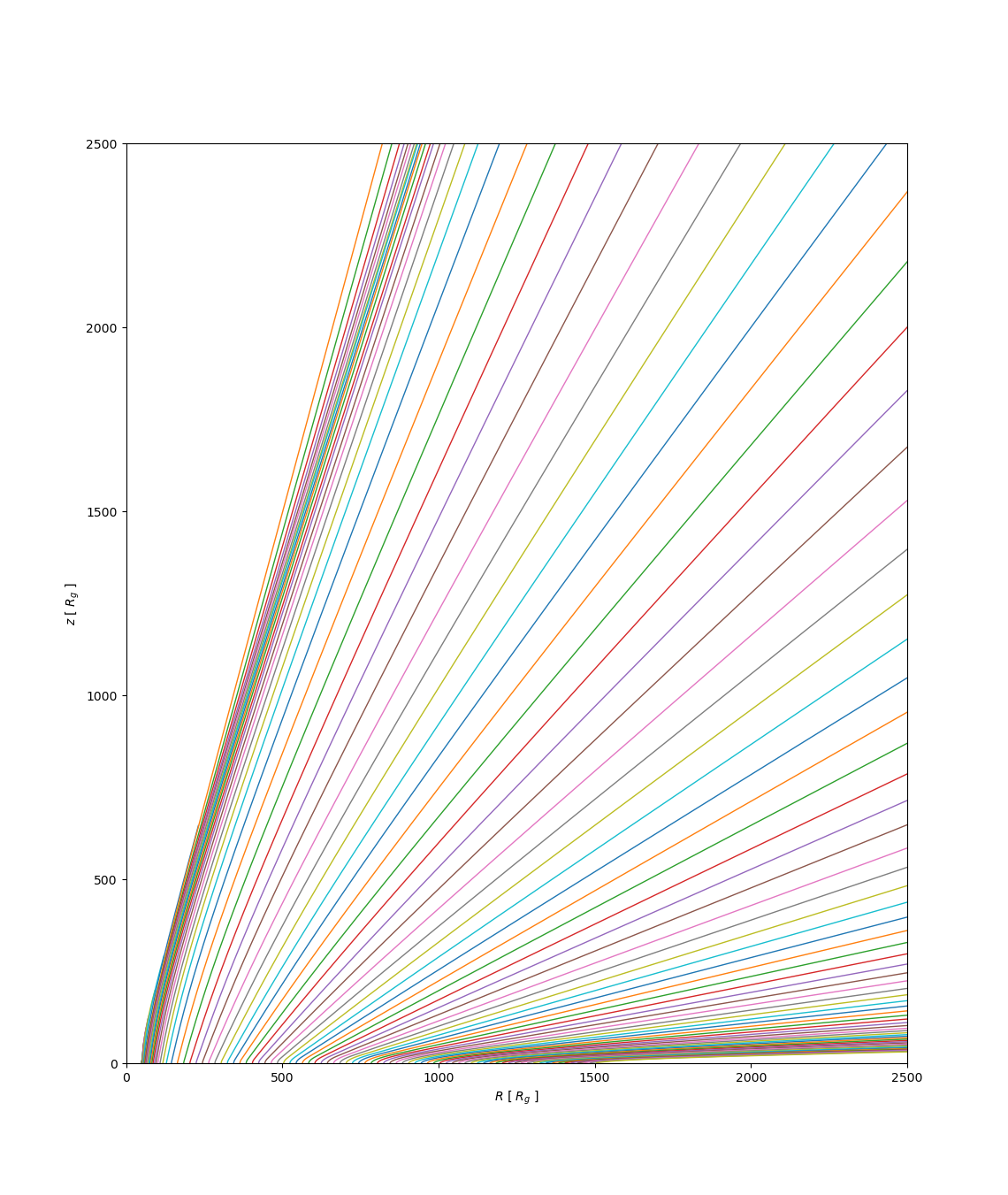

By default, the streamlines of the latest iteration will be loaded. A specific iteration can be checked with

streamlines = Streamlines("example/results.hdf5", 2)

Density Grid

Similarly,

dgrid = DensityGrid("./example/results.hdf5");

LogNorm = matplotlib.colors.LogNorm
fig, ax = plt.subplots()
cm = ax.pcolormesh(dgrid.r_range, dgrid.z_range, dgrid.grid', norm=LogNorm(1e4, 1e8))
plt.colorbar(cm, ax=ax)
ax.set_xlim(0,2500)
ax.set_ylim(0,2500)
ax.set_xlabel(L"$R$ [ $R_g$ ]")
ax.set_ylabel(L"$z$ [ $R_g$ ]")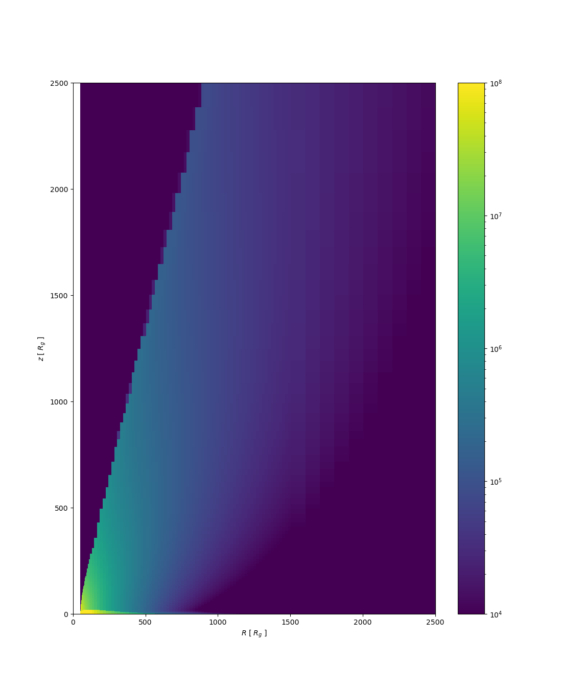

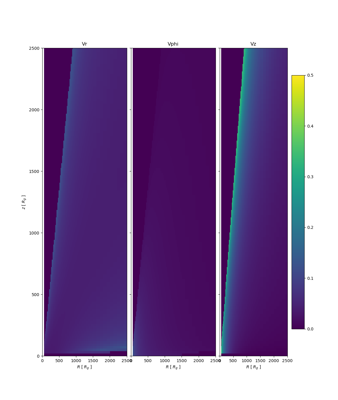
Velocity Grid

Normalize = matplotlib.colors.Normalize
fig, ax = plt.subplots(1, 3, figsize=(6,2), sharex=true, sharey=true)
ax[1].pcolormesh(vgrid.r_range, vgrid.z_range, vgrid.vr_grid', norm=Normalize(0, 0.5))
ax[2].pcolormesh(vgrid.r_range, vgrid.z_range, vgrid.vphi_grid', norm=Normalize(0, 0.5))
cm = ax[3].pcolormesh(vgrid.r_range, vgrid.z_range, vgrid.vz_grid', norm=Normalize(0, 0.5))
plt.colorbar(cm, ax=ax[3])
ax[1].set_ylim(0,2500)
ax[1].set_xlim(0,2500)
for i in 1:3
    ax[i].set_xlabel(L"$R$ [ $R_g$ ]")
end
ax[1].set_ylabel(L"$z$ [ $R_g$ ]")
ax[1].set_title("Vr")
ax[2].set_title("Vphi")
ax[3].set_title("Vz")
plt.subplots_adjust(wspace=0.05, hspace=0.05)