import torch
import numpy as np
import matplotlib.pyplot as plt

Differentiating through randomness

Fixed noise distribution

In the previous notebook (01-automatic-differentiation) we covered the basics of automatic differentiation (AD). However, we left an important detail for ABMs out. How can we compute the derivative of stochastic programs, and what does that mean, exactly?

Consider the following program with an input parameter $\theta$

where $\mathcal N(\mu, \sigma)$ is the Normal distribution with mean $\mu$ and standard deviation $\sigma^2$. This can be coded as:

def f(theta):
    z = np.random.normal(1, 2)
    return theta**2 * (z + 4)

So, what does it mean to compute

If we think about the standard definition of derivative,

we can observe that this is not well defined since the difference $f(\theta+\epsilon) - f(\theta)$ will take random values and it is not clear how to treat this limit.

However, in many cases, we are actually interested in the derivative of an average model realization, not just the derivative of a single run. In other words, we want to take gradients of the form

where $p$ is a probability density and $f$ is a (deterministic) simulator with structural parameters $\theta$. Taking the derivative we have

so that the gradient of the expectation is the expectation of the gradient.

In our considered example, this translates to

now we can take the derivative

Let’s check this result numerically.

theta = 2.0
epsilons = [1.0, 0.5, 0.1]
n_samples = 10_000
samples_per_epsilon = {epsilon: [] for epsilon in epsilons}
for epsilon in epsilons:
    for i in range(n_samples):
        f_deriv = (f(theta + epsilon) - f(theta)) / (epsilon)
        samples_per_epsilon[epsilon].append(f_deriv)

fig, ax = plt.subplots()
for i, (epsilon, samples) in enumerate(samples_per_epsilon.items()):
    ax.hist(
        samples,
        bins=100,
        alpha=0.6,
        label=f"$\epsilon={epsilon}$",
        density=True,
        color=f"C{i}",
    )
ax.axvline(
    theta * 10,
    color="black",
    linestyle="dashed",
    linewidth=1,
    label="Expected derivative",
)
ax.legend()

<matplotlib.legend.Legend at 0x13fcacac0>

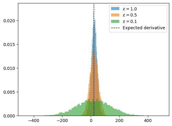
What is going on? The smaller $\epsilon$ is, the variance of our estimator is going $\to \infty$!

This is caused by the fact that the two function calls $X(p)$ and $X(p+\epsilon)$ are uncorrelated (they have a different random seed) and so even calling the program for very similar values of $p$ can cause large differences.

Nonetheless, the finite differences method gives an unbiased estimator.

This issue is not present in automatic differentiation engines, since they only require one evaluation of the model.

def f_torch(theta):
    z = torch.distributions.Normal(1.0, 2.0).sample()
    return theta**2 * (z + 4)


n_samples = 10_000
samples_autograd = []
for i in range(n_samples):
    theta = torch.tensor(2.0, requires_grad=True)
    f_torch(theta).backward()
    samples_autograd.append(theta.grad)

fig, ax = plt.subplots()
ax.hist(
    samples_autograd, bins=100, label="Autograd", density=True, color="C0"
)
ax.axvline(
    10*theta.item(), color="black", linestyle="dashed", linewidth=1, label="Expected derivative"
)
ax.legend()

<matplotlib.legend.Legend at 0x15c053820>

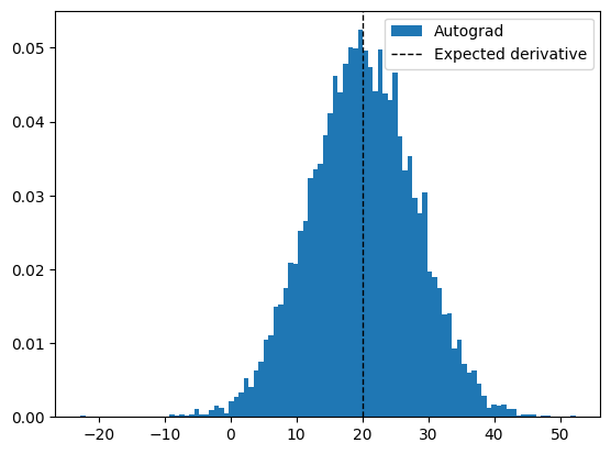
As we can see, the variance is much lower than the finite difference case.

Parameterizable noise

In the example above, we made the assumption that the randomness of our model $p(z)$ did not depend on the structural parameters $\theta$ that we want to differentiate by.

However, in most agent-based models this assumption does not hold. Consider, for instance, the case of an SIR model where agents become infected with some probability $q$. This probability may depend on structural parameters such as $R_0$ or social distancing measures that we want to calibrate.

So now we have

where $p$ is parameterized by $\theta$. Expanding the same way as before we find

notice that now we have an additional term, $\int_z f_\theta(z) \nabla_\theta p_\theta(z) \mathrm{d} z$, that prevents us from commuting the gradient and the expectation. So, in general, the gradient of the expectation is not the expectation of the gradient when our structural parameters parameterize the randomness.

The reparameterization trick

To circumvent this, we introduce the reparameterization trick. Continuous distributions have a property that allows an indirect way of sampling from them. One is direct sampling

and indirectly,

where $g$ is a deterministic path that maps parameter-free noise ($\epsilon$) to $x$. For instance, to sample from a Normal distribution $\mathcal N(\mu, \sigma^2)$, we can do

What have we accomplished with this? We have untangled the “random” part of the distribution from the part that depends on the parameters. This allows us to re-formulate (1) as

where now we can move the gradient inside,

So we have been able to transform the gradient of the expectation to the expectation of the gradient. This can be computed provided that $f$ and $g$ are differentiable. This expectation can now be estiated by Monte Carlo,

Let’s see an example. Consider the program with input $\theta$

The expected answer is

Let’s first check both the parameterized and unreparameterized version:

def f_torch_norep(theta):
    z = torch.distributions.Normal(theta, 2.0).sample()
    return theta**2 * (z + 4)


def f_torch(theta):
    epsilon = torch.distributions.Normal(0, 1).sample()
    z = theta + epsilon * 2
    return theta**2 * (4 + z)


rep_samples = []
norep_samples = []
n_samples = 2_000
theta_value = 2.0
analytical_result = 8 * theta_value + 3 * theta_value**2
for i in range(n_samples):
    theta = torch.tensor(theta_value, requires_grad=True)
    f_torch_norep(theta).backward()
    norep_samples.append(theta.grad.item())
    theta = torch.tensor(theta_value, requires_grad=True)
    f_torch(theta).backward()
    rep_samples.append(theta.grad.item())

fig, ax = plt.subplots()
ax.hist(
    norep_samples,
    bins=100,
    alpha=0.35,
    label="No Reparametrization",
    density=True,
    color="C0",
)
ax.hist(
    rep_samples,
    bins=100,
    alpha=0.35,
    label="Reparametrization",
    density=True,
    color="C1",
)
ax.axvline(
    analytical_result,
    color="black",
    linestyle="dashed",
    linewidth=1,
    label="Expected derivative",
)
ax.legend()

<matplotlib.legend.Legend at 0x14fdd8280>

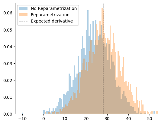
As we can see, we need to be careful, because PyTorch may not be applying the reparameterization trick and we may obtain the wrong results!!

By calling dist.sample() the gradient propagation stops and so we obtain the wrong result. Thankfully, PyTorch has a shortcut to implement the reparameterization trick for us so we don’t have to do it manually. This can be done by using the .rsample() method.

def f_torch(theta):
    z = torch.distributions.Normal(theta, 2.0).rsample()
    return theta**2 * (z + 4)


rep = (
    sum([torch.func.grad(f_torch)(torch.tensor(2.0)) for i in range(n_samples)])
    / n_samples
)
print(f"{rep} ~ {analytical_result}")

27.93507194519043 ~ 28.0

A note on reinforcement learning

Recall equation (1):

There is an alternative way to re-express this gradient:

The familiar reader will recognize the last expression as the score-based estimator of the gradient, also known as REINFORCE in the RL community. The advantage of calculating the gradient this way, is that we only require the density $p$ to be differentiable, but we have no constraints on $f$. However, this gradient does not scale well for high dimensionality of $\theta$, compared to the path-wise approach, since the variance scales with the dimension of $\theta$. See this reference for an in-depth review.

Discrete randomness

The above discussion about the reparameterization trick makes the assumption that the probability density is differentiable. This is true for continuous distributions but it does not hold for discrete ones such as Bernoulli or Categorical distributions.

Multiple methods exist to deal with this issue, the most common ones being the Stright-Through estimator (Bengio et al. 2013) or the Gumbel-Softmax trick (Jang et al. 2016). Newer methods are continuously being developed such as the StochasticAD.jl package in the Julia language.

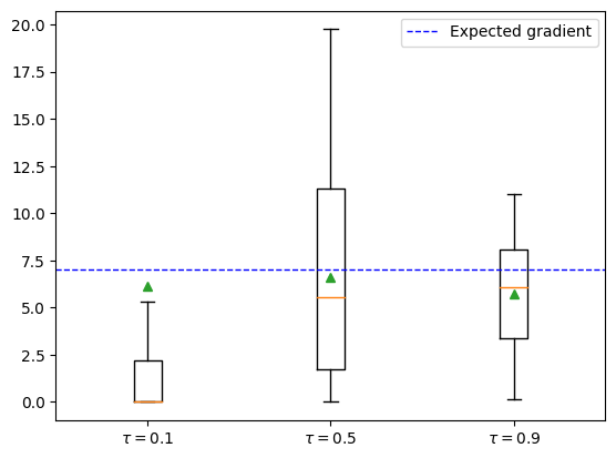
Here, we focus on the Gumbel-Softmax (GS) trick. The GS distribution is a continuous relaxation of the Categorical distribution. The GS has a temperature parameter $\tau$ which controls the smoothness of the approximation such that the exact Categorical sampling is recovered for $\tau\to 0$. However, the variance of the gradient will grow as $\tau\to 0$ so $\tau$ acts as a bias-variance trade-off.

PyTorch has a standard implementation ready to use. In particular, it implements a “hard” version of GS. The idea is that we can use the samples from the categorical distribution in the forward simulated pass, and use the continuous relaxation to approximate the gradients in the backward pass. This way we guarantee that the forward simulation is exactly equivalent to the non-relaxed version.

Consider the program with input parameter $\theta$:

We have

def sample_bernoulli(theta, gs_tau):
    logits = torch.cat([theta, 1 - theta]).log()
    return torch.nn.functional.gumbel_softmax(logits=logits, tau=gs_tau, hard=True)


def f(theta, gs_tau):
    return 2 * sample_bernoulli(3 * theta, gs_tau) + sample_bernoulli(theta, gs_tau)

n_samples = 1_000
taus = [0.1, 0.5, 0.9]
gradients_per_tau = {}
for tau in taus:
    gradients = []
    for i in range(n_samples):
        theta = torch.tensor([0.1], requires_grad=True)
        f(theta, tau)[0].backward()
        gradients.append(theta.grad.item())
    gradients_per_tau[tau] = gradients

fig, ax = plt.subplots()
for i, (tau, gradients) in enumerate(gradients_per_tau.items()):
    ax.boxplot(gradients, showmeans=True, positions=[i], labels=[f"$\\tau={tau}$"], showfliers=False)
ax.axhline(7, color="blue", linestyle="dashed", linewidth=1, label="Expected gradient")
ax.legend()

<matplotlib.legend.Legend at 0x15c2efe20>